Master Datasheets
Data from downed woody debris was placed in R where each transect line used the sum of the diameters (Marshall et al. 2000) and then the average of all 6 transect lines were found to estimate the total volume of each plot. The volume of the standing dead was calculated using estimated heights and using the estimate volumes of trees based on DBH from Ecologically based individual tree volume estimation for major Alberta tree species.
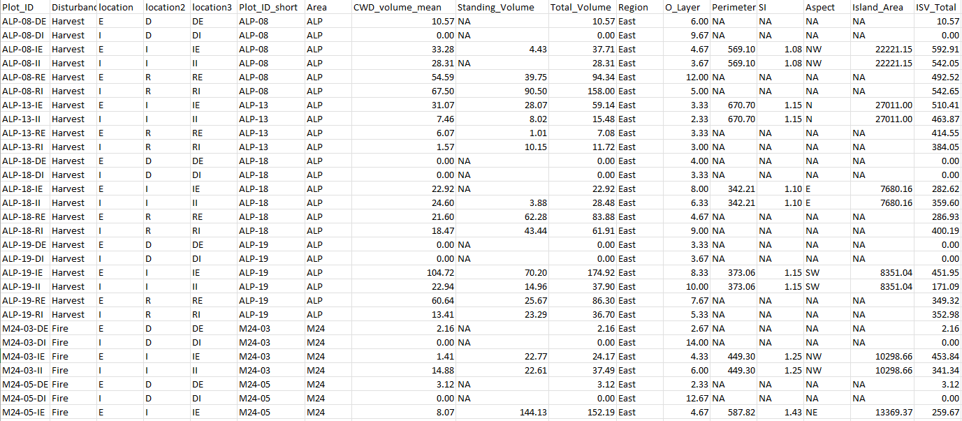
Table 1. Data set for coarse woody debris after volume calculations.
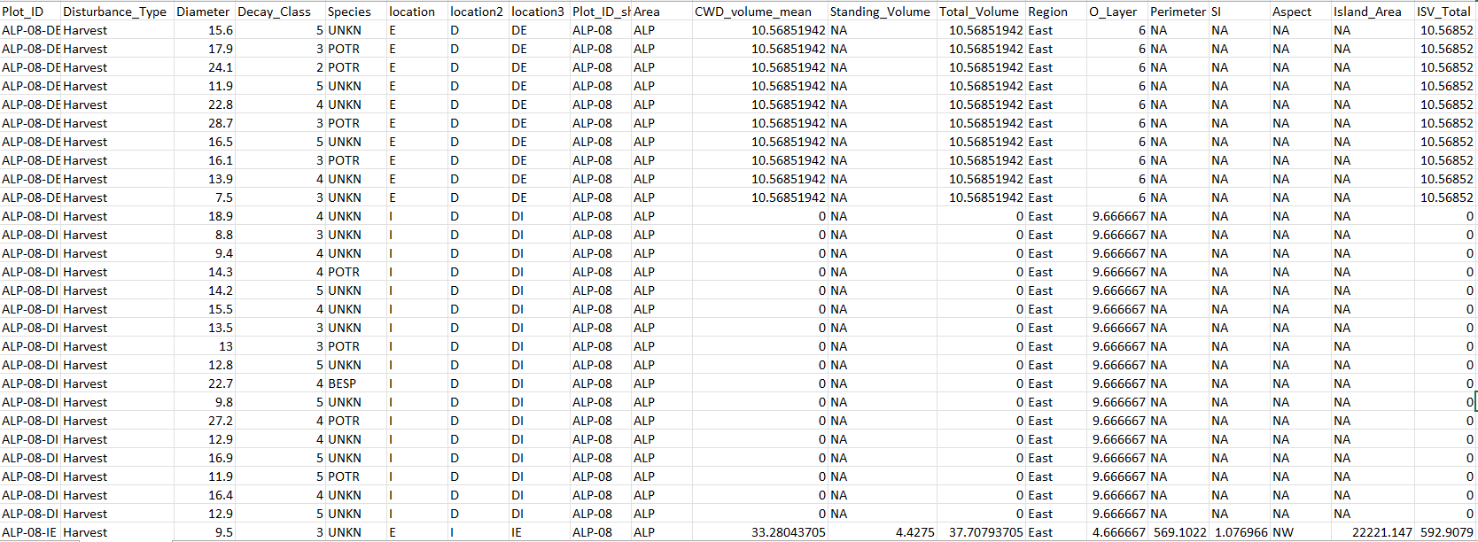
Table 2. Data set for each piece recorded.
Attribute and Site Variables
Plot ID: Unique plot name
Disturbance Type: Type of disturbance the plot experienced or was adjacent
Location: Interior or edge of a disturbed, reference or island area
Location 2: The disturbed, reference or island area
Location 3: The specific area in a plot, such as reference edge or disturbed interior
Area: 1 of 6 geographical locations the survey was taken [MEE (Mercer Harmon Valley), MEW (Mercer West), ALP (Alpac), M24 (M024 Fire Complex), S56 (S056 Fire Complex) and S57 (S057 Fire Complex)]
CWD Volume Mean: Downed coarse woody debris volume estimate, according to line-intercept method calculations (m3/ha)
Standing Dead: Standing coarse woody debris volume estimate, according to Alberta species-specific volume calculations (m3/ha)
Total Volume: Sum of downed and standing coarse woody debris
Region: Geographical portion of Alberta the plots are located (East vs West)
Organic Layer: Mean of organic layer depth at each plot (centimeters)
Perimeter: Length of the periphery of the island (meters)
Shape Index: Perimeter/(square root(pi*area))
Aspect: Cardinal direction location of plots within an island
Island Area: Amount of surface in each island (meters squared)
Initial Stand Volume: The sum of the volumes of the living trees and the dead trees (standing and dead) of decay class 1 & 2
Diameter: Diameter of coarse woody debris that was recorded (centimeters)
Decay Class: Decomposition classification of coarse woody debris recorded (1-5)
Species: Species of each coarse woody debris piece
Exploratory Plots

Plot 1. Boxplots display the total coarse woody debris volume of decay classes 1-5 between harvests and fires, separated by plot location.
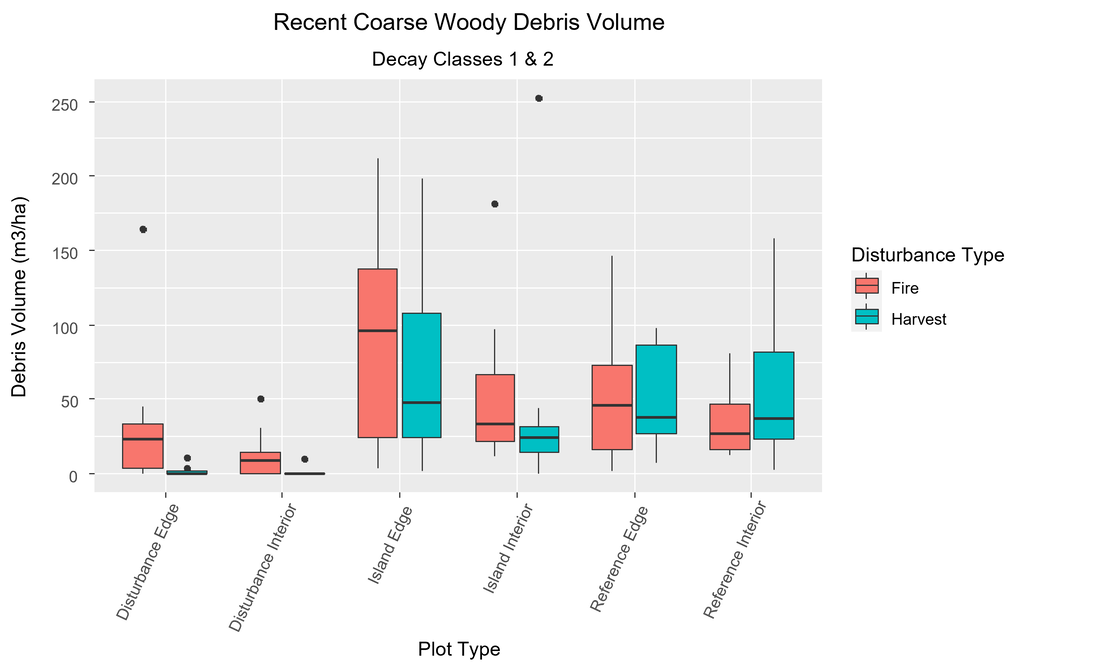
Plot 2. Boxplots show coarse woody debris volumes of decay classes 1 and 2 compared between harvests and fires, according to the plot location.
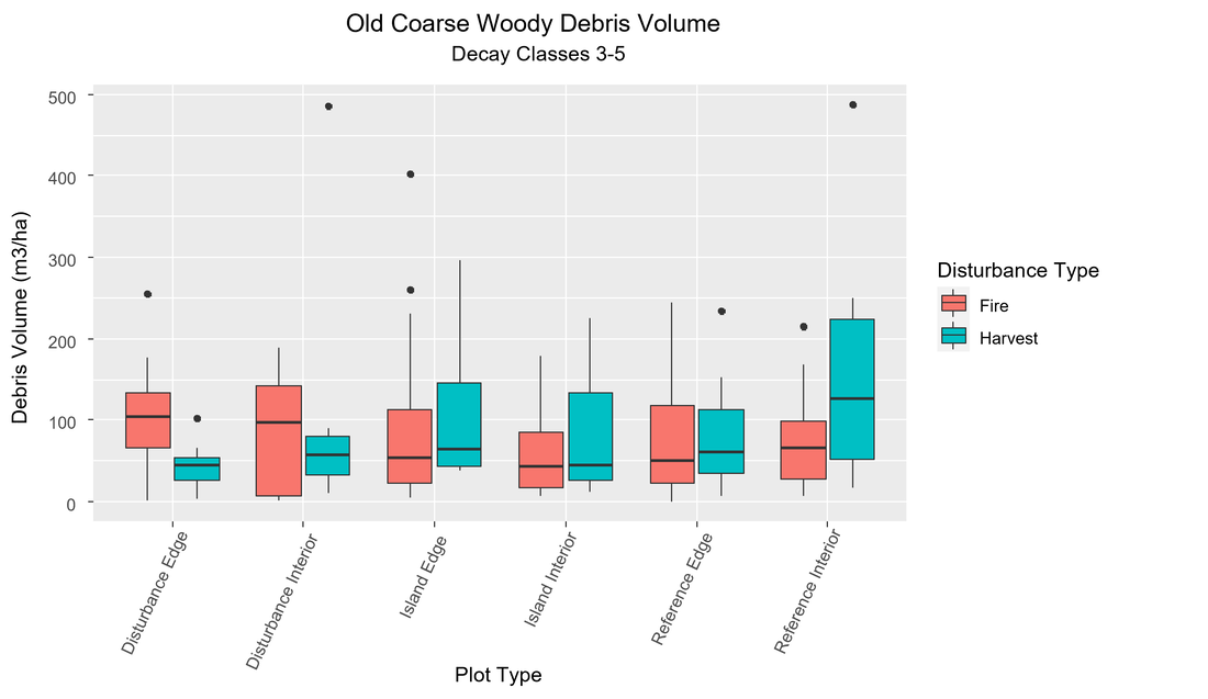
Plot 3. Boxplots show coarse woody debris volumes of decay classes 3-5 compared between harvests and fires, according to the plot location.
Plots 1-3 display the coarse woody debris volume depending on the type of decay class. Because the focus of our project is on disturbances that occurred around a decade ago the older decay classes (3-4) are not going to be analyzed further. The relationship we can see between different sites might be due more to older decay classes, but because we did not investigate older disturbances we are unable to determine their influences. As for the recent coarse woody debris comparison, the disturbances for fire had a larger amount of debris volume due to the methods of harvesting removal of a majority of woody material within the harvesting zone. Looking at the islands it is apparent that there is a larger amount of debris volume in island edges of fires compared to harvests and little variation for island interiors. This is likely due to the characteristics of fires. In creating an island fires often drop from canopy to surface creating a gradient edge. In sampling the true edge is more convoluted than with a harvest, so it is likely that the larger volume of deadwood is due to edge placement and fire characteristics. Another possibility is the fires still had standing dead trees in the disturbance edge plots, so it is possible for those trees to fall into the island edge plot and be double counted. This is not possible with harvests because of the lack of trees in the disturbance areas. Lastly, the reference areas showed little variation between fire and harvest sites.
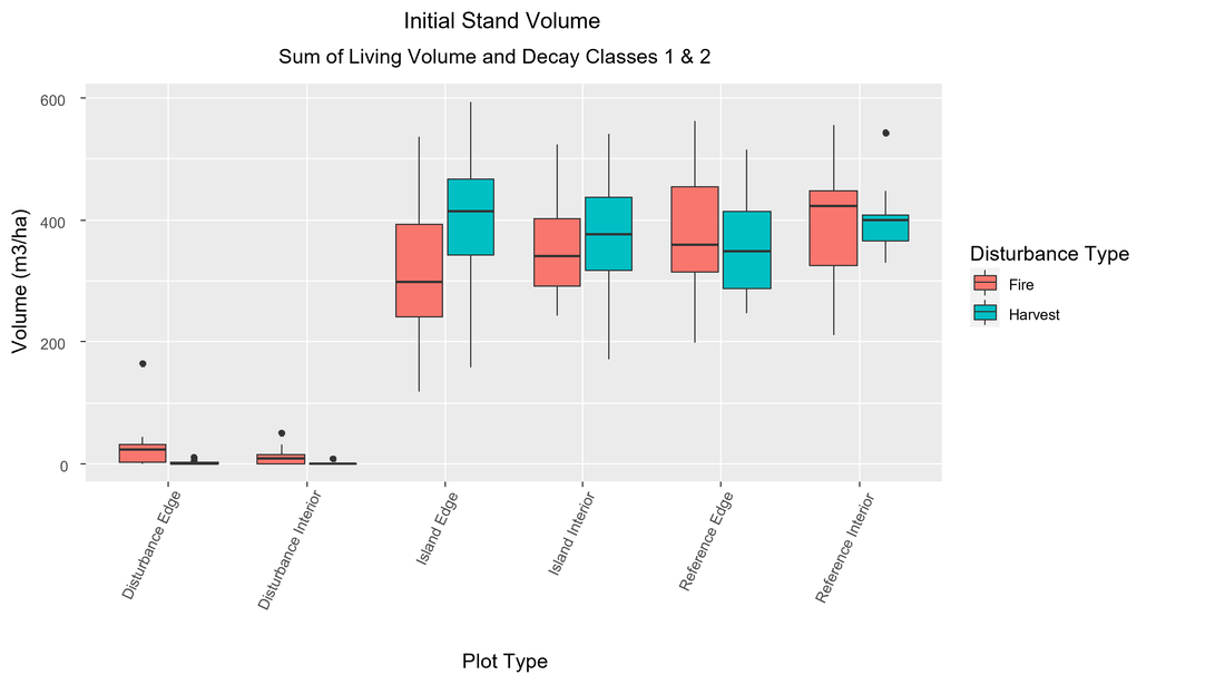
Plot 3. Boxplot comparison of the initial stand volume between harvests and fires, according to plot location. Initial stand volume was calculated by summing the living tree volumes and the dead decay classes 1 & 2.
The initial stand volume was calculated to identify if deadwood accumulations corresponded to overall density of the plots before the disturbance. The harvest disturbed areas were impossible to calculate because the method I used required interpretation from preexisting downed and standing trees. Nevertheless, the islands and references provided more accurate depictions. Interestingly, the island edges of fires presented lower initial stand volumes even though they presented higher deadwood volumes. As for the island interiors, reference interiors and reference edges, there is little variation amongst the disturbance types.
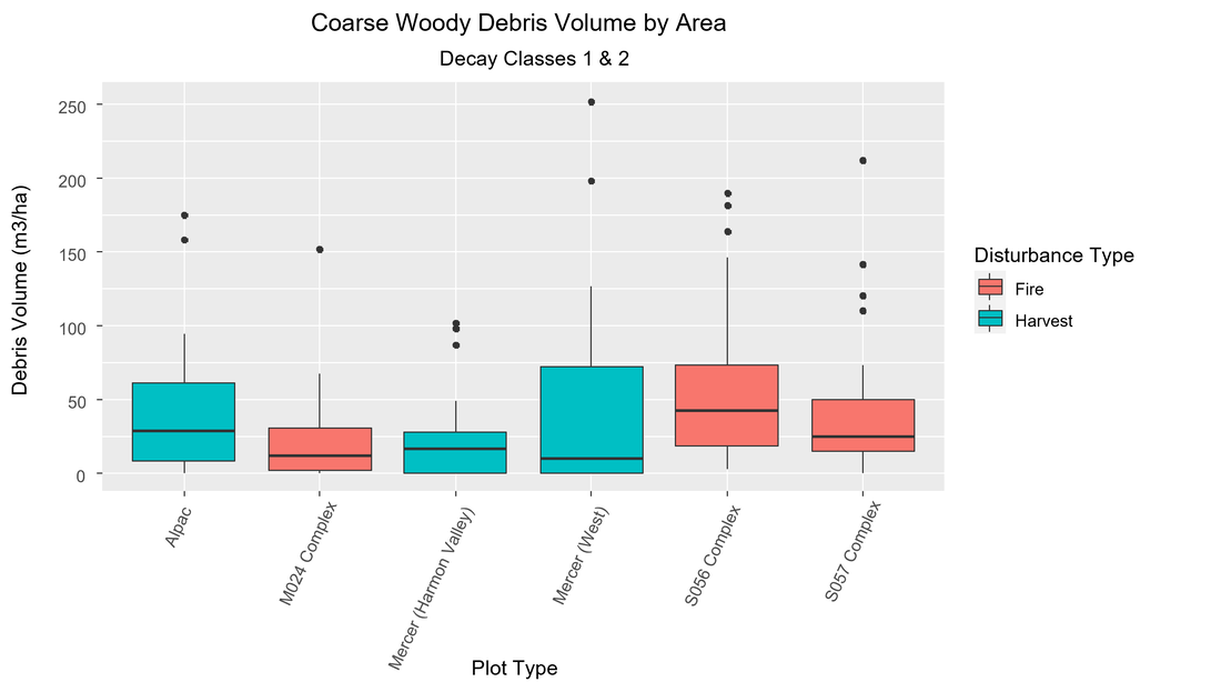
Plot 4. Boxplot of coarse woody debris volume (decay classes 1 and 2) by geographical location.
In Plot 4 I wanted to see how each area compared to one another in terms of debris volume. Even comparing the lowest area to the highest there is only ~30 m3/ha difference between the two. The harvest and fire areas do not seem to display a pattern either.
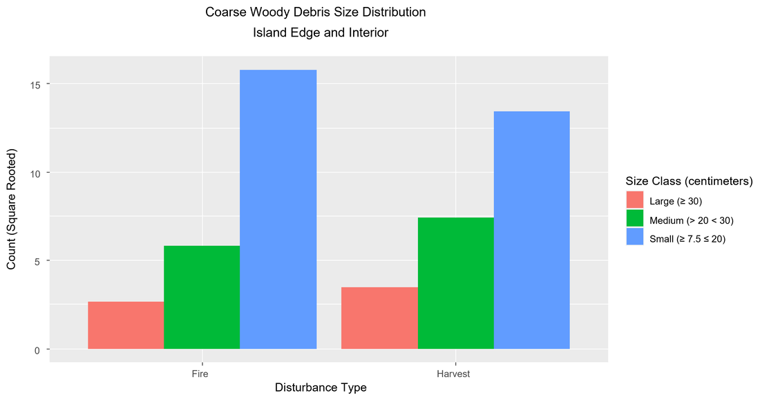
Plot 5. Bar graph displaying the distribution of coarse woody debris sizes between harvests and fires.
Plot 5 is used to show how diameter distributions compare between the two disturbance types. The diameters are labelled as small, medium and large to give an idea about the type of ecological functions available in each disturbance type. Larger diameter debris are able to support more biodiversity and aid in rare species habitat creation. Fires, overall, have more logs within the islands, but harvests possess more in the medium and large classifications. The variation is not enough to warrant too much of a distinction, but enough to state that the type of disturbance does not drastically alter the diameter size of the debris in island remnants.
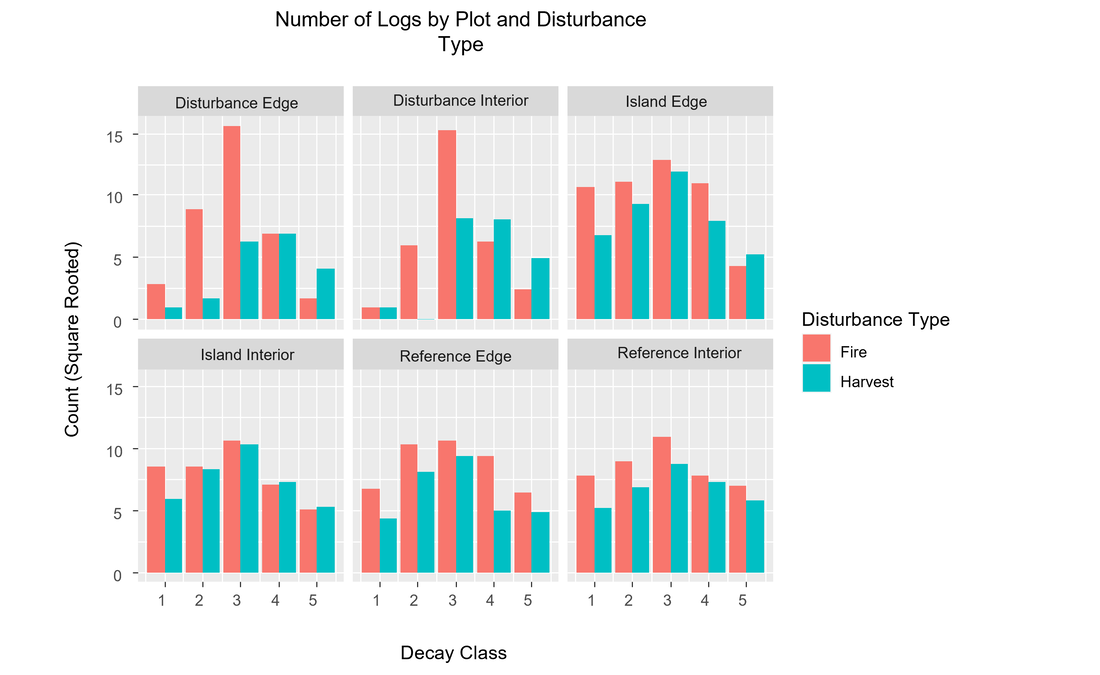
Plot 6. Bar graph comparing the amount of coarse woody debris pieces in each plot location between harvests and fires.
This plot is used to visualize the distribution of debris across decay classes and plots. The disturbance areas of fires show a greater amount of pieces in the early decay classes because the harvesting methods removed all of the young logs on the harvest areas. The island and reference areas show little variation as well. Fires are slightly higher in these situations, but not dramatically.
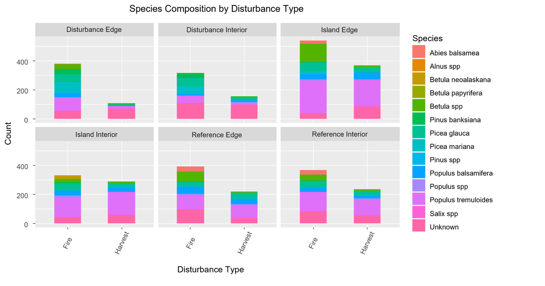
Plot 7. Stacked bar graph displaying the species composition of the dead trees between harvests and fires, according to the plot location.
The species composition plot shown in Plot 7 was used to display how species might change based on disturbance type and plot location. Looking at the island and reference plots one can see that Betula spp. and Abies spp. tended to be present in fire plots more so than harvest plots. This information is hard to utilize due to the large number of unknowns from the inability to identify decayed species.
